Introduction to volatility models with Matlab (Implied volatility)

Implied volatility (IV) is the volatility of an asset derived from changes in value of corresponding option in such way that if we input IV into option pricing model, it will return theoretical value equal to the current option value. Contrary to historical volatility, IV is the volatility forecast for price of the underlying asset from current time $t$ to option expiration $T$ . Let’s quickly introduce the Black-Scholes option pricing model. There are multiple ways to derive BSE and you can review them here. The brief solution of BSE can be found here. So the familiar BSE form is

(1) $\begin{equation*} \frac{\partial V}{\partial t} + \frac{1}{2}\sigma^2 S^2 \frac{\partial^2 V}{\partial S^2} + rS\frac{\partial V}{\partial S} - rV = 0 \end{equation*}$

where

$V$ – option value,
$S$ – underlying asset spot price,
$r$ – risk-free interest,
$t,T,T-t$ – current time, date of expiry, time to expiry,
$\sigma$ – volatility (in our case implied volatility).

The solution of (1) for value of an call or put option at time $t<T$ can be expressed as

(2) $\begin{equation*} C_t = S_t\Phi(d_1) - Ke^{-r(T-t)}\Phi(d_2),\hspace{10pt} P_t = Ke^{-r(T-t)}\Phi(-d_2)-S_t\Phi(-d_1) \end{equation*}$

where

$d_1 = \frac{ln \big(\frac{S_t}{K}\big) + (r+\frac{1}{2}\sigma_t^2)(T-t)}{\sigma_t\sqrt{T-t}} ,$

$d_2 = d_1 - \sigma_t \sqrt{T-t} ,$

$K$ is strike price of an option and $\Phi$ is value of normal CDF at particular points $d_1,d_2$ . Recall that normal CDF is written

$\Phi(d) = \frac{1}{\sqrt{2\pi}}\int_{-\infty}^d \! exp\Big(-\frac{y^2}{2}\Big) \, \mathrm{d}y.$

Do you see how deeply $\sigma_t$ is buried? We see that $\Phi(d_1(\sigma_t))$ and $\Phi(d_2(\sigma_t))$ and since there doesn’t exist the closed form solution of $\Phi(d)$ the $\sigma_t$ can’t be expressed analytically. That’s why we use numerical methods and approximation to evaluate implied volatilities. Familiar widely used numerical approaches are Newton-Raphson or secant method. Approximation of IV can be estimated by Bharadia-Christopher-Salkin(1996) model or Corado-Miller(1996) model. Among the latest and most effective estimators we can sort Hallerbach(2004), Jaeckel(2006) and Jaeckel(2013).

For purpose of this article let’s show how to implement just the most basic B-C-S model and secant method.

The B-C-S model is derived as

(3) $\begin{equation*} \sigma_t = \sqrt{(2\pi-(T-t))}\Big(\frac{V_t-\delta}{S_t-\delta}\Big),\hspace{10pt}\delta = \frac{1}{2}(S_t-Ke^{-r(T-t)}) \end{equation*}$

where

$T-t$ – time to option expiration,
$V_t$ – current option value,
$S_t$ – underlying asset spot price,
$K$ – option strike price( $Ke^{-r(T-t)$ is discounted strike price).

The secant numerical method is given by

(4) $\begin{equation*} \sigma_{i+1} = \sigma_i - (BS(\sigma_i) - V_t)\bigg[\frac{\sigma_i - \sigma_{i-1}}{BS(\sigma_i) - BS(\sigma_{i-1})}\bigg] \end{equation*}$

where

$BS(\sigma_i)$ is theoretical option value from (2).

Algorithm itself works as follows(suppose $\sigma$ computation for one specific $t$ ):

Compute $\sigma_{BCS}$ using (3).
Compute theoretical value of an option $BS(\sigma_{BCS})$ using (2).
Set initial values(initial guess) for secant method, that is $\sigma_{i-1}=0,\hspace{5pt}\sigma_{i}=\sigma_{BCS}$
and $BS(\sigma_{i-1})=0,\hspace{5pt}BS(\sigma_{i})=BS(\sigma_{BCS})$ .
These temporary variables will change in the secant method loop. Keep in mind that the iterator in (4) of the secant loop is $i$ (not $t$ !).
Compute approximation error(last product on the left side of (4)).
Compute new $\sigma_{i+1}$ using (4).
Compute new $BS(\sigma_{i+1})$ using (2)
If error < accuracy threshold then last $\sigma_{i+1}$ is our $\sigma$ from secant method alias implied volatility. Proceed to the next $t$ .
If error is > accuracy threshold go back to step 6 (proceed to the next $i$ ) and don’t forget you need to recompute new $BS(\sigma_{i+1})$ values. Use $\sigma_{i+1}$ from last secant iteration (note that initial values from step 3. and 4. will not be used in 2nd secant iteration). On every new iteration, $i$ variables become $i-1$ variables and new $i+1$ variables are computed.

I will use historical EOD option chain data for BAC stock.

BAC2015_option_chain
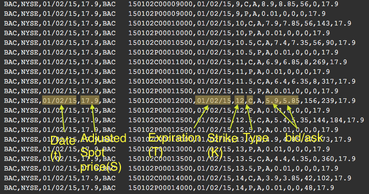
Fig.3 Example option chain .csv file for BAC stock.

If you are wading through my intro to volatility thoroughly you may want to download the example option chain. Option data are very expensive and tough to store and manipulate so it’s nearly impossible to find them free. So now we need to prepare data for IV calculation as follows:

Use optionparse() function for importing the .csv option chain into matlab table.

 table = optionparse('path/to/datafile','ivolatility','equity');

Now we extract dates $t$ , adjusted stock spot prices $S$ and we choose call options with strike $K=15$ , time to expiry $T-t = 0.5$ and the ‘risk-free’ interest rate be $r=0.001$ which was T-Bill rate in the early 2015. Let me point out that in practice $T-t$ “constant” will not be constant because we will not find such options at every time $t$ which have exactly half a year expiration. Only finite number of options is offered every $t$ . So our $T-t$ will be variable. At every $t$ I choose the first option with $T-t > 0.5$ and $K = 15$ . Following code finds forementioned options.

% find dates
[~,ia,ib] = unique(table.data.date,'first','legacy');
t = table.data.date(ia);
S = table.data.adjusted_stock_close_price(ia);

% time to expiration in N/252 fraction, for simplicity I don't consider holidays, in practice you should
Tte = yearfrac(table.data.date,table.data.expiration,13);

% search options with expiration T_t and strike K
T_t_const = 0.5;
K = 15;

% expiration filter
ic_start = ia + accumarray(ib,Tte,[],@(x) find(x>=T_t_const,1)) - 1;
ic_end = ia + accumarray(ib,Tte,[],@(x) find(x<=T_t_const+0.5,1,'last')) - 1;
idExpiration = zeros(size(Tte));

% strike filter
id = zeros(length(ic_start),1);
for i=1:length(ic_start)
    temp = find(table.data.strike(ic_start(i):ic_end(i)) == K,1);
    if ~isempty(temp)
        id(i,1) = find(table.data.strike(ic_start(i):ic_end(i)) == K,1);
    else
        id(i,1) = NaN;
    end
end

% uncomment proper option
idTK = ic_start + id - 1; % call options
% idTK = ic_start + id; % put options

% time to expiry at each time t
T_t_var = Tte(idTK);

% let the value of the option be (ask+bid)/2. V is vector with filtered
% options
V = (table.data.ask(idTK) + table.data.bid(idTK))/2;

Our variables and constants are ready. I will demonstrate IV computation for $t=1$ .

1. Calculate initial IV estimate $\sigma_{BCS}$ by B-C-S model (3).

t = 1;
r = 0.001;
delta = (1/2)*(S(t) - K*exp(-r*T_t_var(t))); % (3)
sigma_BCS(t,1) = sqrt(2*pi-T_t_var(t)) * (V(t)-delta)/(S(t)-delta); % (3)

2. Compute theoretical value of an option $BS(\sigma_{BCS})$ using (2).

d1 = (log(S(t)/K) + (r+1/2*sigma_BCS(t,1)^2)*(T_t_var(t))) / sigma_BCS(t,1)*sqrt(T_t_var(t)); % (2)
d2 = d1 - sigma_BCS(t)*T_t_var(t);
BS(t) = S(t)*cdf('normal',d1,0,1) - K*exp(-r*T_t_var(t))*cdf('normal',d2,0,1); % (5) for call option

3. Set initial values(initial guess) for secant method, that is $\sigma_{i-1}=0,\hspace{5pt}\sigma_{i}=\sigma_{BCS}$ . Note that I smuggled in the initial error value and secant method accuracy.

err_thr = 1e-4; % secant method error tolerance(accuracy)
err = 1; % initial error value
temp_sigma(1:2,1) = [0,sigma_BCS(t,1)];

4. and $BS(\sigma_{i-1})=0,\hspace{5pt}BS(\sigma_{i})=BS(\sigma_{BCS})$ .

temp_BS(1:2,1) = [0,BS(t,1)];

5. Secant method, steps described in the code.

while err >= err_thr
                
    % error update - step 6
    err = (temp_BS(2,1) - V(t)) * ... 
        ((temp_sigma(2,1) - temp_sigma(1,1)) / (temp_BS(2,1) - temp_BS(1,1))); % (7) error corresponding to last computed sigma
                
    % sigma_{i+1} update - step 7
    temp_sigma(3,1) = temp_sigma(2,1) - err; % new sigma from secant iteration
    temp_sigma(1) = []; % old sigma no more needed in next loop
                
    % BS(sigma_{i+1}) update - step 8
    d1 = (log(S(t)/K) + (r+1/2*temp_sigma(2,1)^2)*(T_t_var(t))) / temp_sigma(2,1)*sqrt(T_t_var(t)); % (2)
    d2 = d1 - temp_sigma(2,1)*T_t_var(t); % (2)
    temp_BS(3,1) = S(t)*cdf('normal',d1,0,1) - K*exp(-r*T_t_var(t))*cdf('normal',d2,0,1); % (2) for call option
    temp_BS(1) = []; % old BS(sigma) no more needed in next loop
                
end

9. If error < accuracy threshold then last $\sigma_{i+1}$ is our $\sigma$ .

sigma_secant(t,1) = temp_sigma(2,1);

10. If error > accuracy threshold go to step 6 (next $i$ ).

You can download complete working BCS_secant() function here.

secantIV2

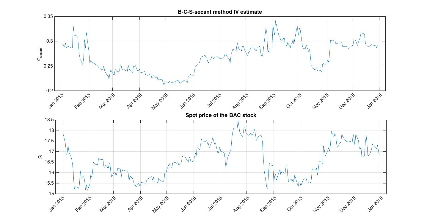
Fig.4 B-C-S-secant computed daily implied volatility for Bank of America stock in 2015

We can slowly move to the next concept of practical importance which ensues directly from implied volatility calculation. We have computed one IV value for every $t$ and we supposed that $\sigma_{secant}=f(T-t,K,.)$ where $T,K$ were fixed (“fixed” for $T$ because $T$ cannot be strictly constant). Clearly we can release this assumption and let the $T,K$ be variables. For every $t$ we now have not just one point but set of points which constitutes the implied volatility surface. If we now fix just $T$ at some time $t$ in $\sigma_{secant}=f(T-t,K,.)$ we obtain values constituting implied volatility smile or implied volatility skew, if we fix just $K$ at some time $t$ we obtain implied volatility term structure.

Multitudes of volatility indexes (composites) are constructed using various setups in IV computation. Some of them average IV’s of stocks in indexes such a S&P500, DJIA, NASDAQ …, some of them average similar ETF’s etc. As was mentioned before such indexes measure expectation of volatility. For example have a look at the CBOE volatility indexes overview.

MMquant

Introduction to volatility models with Matlab (Implied volatility)

Leave a Reply Cancel Reply