Introduction to volatility models with Matlab (ARCH, GARCH, GJR-GARCH)

In this article you get familiar with basic concepts behind GARCH models family and practical use of it.

General properties, terms and notation of conditional variance models

Advantage of conditional variance models is that they better describe following time series properties:

Returns of an asset have positive excess kurtosis^[1] which means their PDF peak is sharper than the normal PDF peak. Tails of returns PDF often embody higher probability density than PDF shoulders, such the PDF has well-known fat-tails.
Volatility tends to cluster into periods with higher and lower volatility. This effect means that volatility at some time must be dependent on its historical values say with some degree of dependence.
Returns fluctuations have asymmetric impact on volatility. Volatility changes more after downward return move than after upward return move.

Consider the general form of conditional variance model

(1) $\begin{equation*} y_t = \mu_t + e_t\>,\hspace{5pt} e_t = \sigma_t \>\varepsilon_t \hspace{5pt}. \end{equation*}$

Firstly we see that value of dependent variable $y_t$ consists of mean $\mu_t$ and innovation $e_t$ . In practice $\mu_t$ can be chosen as conditional mean of $y_t$ such that $\mu_t = E(y_t|\Omega_{t-1})=g(\Omega_{t-1})$ where $\Omega_{t-1}$ ^[2] is arbitrary historical information affecting value of $y_t$ . In other words we model every $\mu_t$ by suitable linear regress model or using AR^[3] process. Often is sufficient use just fixed value $\mu_t=\mu$ or $\mu_t=0$ . Innovation $e_t$ consists of variance(volatility) root $\sigma_t$ where $\sigma_t^2 = h_t = h(\Omega_{t-1}) = var(e_t|\Omega_{t-1}) = var(y_t|\Omega_{t-1})$ ^[4] and i.i.d. random variable from normal or $t$ -distribution $\varepsilon_t \sim N(0,1)$ or $\varepsilon_t \sim t(\nu)$ .

From fragmented notation above we can write general conditional variance model as is known in econometrics literature

(2) $\begin{equation*} y_t = \mu_t + \sigma_t\>\varepsilon_t = \mu_t + \sqrt{h_t}\>\varepsilon_t = g(\Omega_{t-1}) + \sqrt{h(\Omega_{t-1})}\>\varepsilon_t \hspace{5pt}. \end{equation*}$

Observe that innovations $e_t$ are not correlated but are dependent through $\sigma_t$ term (later we will briefly see $\Omega_{t-1}$ contains lagged $\sigma_t^2$ ). If $g$ is non-linear function then model is non-linear in mean, conversely if $h$ is non-linear then model is non-linear in variance which in turn means that $h_t$ is changing non-linearly with every $t$ through a function of $\Omega_{t-1}$ . Since now we should know what autoregressive conditional heteroskedasticity means.

ARCH

After discussion above we can quickly formulate the ARCH model which was introduced by Rober Engle in 1982. If we take (2) and specify condition(based on historical information $\Omega_{t-1}$ ) for $\sigma_t$ we get ARCH(m) model

(3) $\begin{equation*} y_t = \mu_t + e_t \>,\hspace{5pt} e_t = \sigma_t\>\varepsilon_t\>,\hspace{5pt}\sigma_t^2 = \underbrace{\alpha_0 + \sum \limit_{\tiny i=1}^{\tiny m} \alpha_i \> e_{t-i}^2}_{condition} \end{equation*}$

where $\varepsilon_t$ are i.i.d. random variables with normal or $t$ -distribution, zero mean and unit variance. As mentioned earlier in practice we can drop $\mu_t$ term thus get

$y_t = e_t \>,\hspace{5pt} e_t = \sigma_t\>\varepsilon_t\>,\hspace{5pt}\sigma_t^2 = \alpha_0 + \sum \limit_{\tiny i=1}^{\tiny m} \alpha_i \> e_{t-i}^2$

or regress mean with exogenous explanatory variables as

$y_t = \underbrace{\gamma_0 + \sum \limit_{\tiny i=1}^{\tiny k}\gamma_i \>x_{t,i}}_{\mu_t} \>+\> e_t \>,\hspace{5pt} e_t = \sigma_t\>\varepsilon_t\>,\hspace{5pt}\sigma_t^2 = \alpha_0 + \sum \limit_{\tiny i=1}^{\tiny m} \alpha_i \> e_{t-i}^2$

or use any other suitable model. Recall that significant fluctuation in past innovations will notably affect current volatility(variance). Regarding positivity and stationarity of variance $\sigma_t^2$ , coefficients in (3) condition have to satisfy following constraints

$\alpha_0 > 0,\>\alpha_1 \ge 0,\>\cdots ,\>\alpha_m \ge 0,\hspace{5pt} \sum \limit_{\tiny i=1}^{\tiny m} \alpha_i < 1$

GARCH

GARCH model was introduced by Robert Engle’s PhD student Tim Bollerslev in 1986. Both GARCH and ARCH models allow for leptokurtic distribution of innovations $e_t$ and volatility clustering (conditional heteroskedasticity) in time series but neither of them adjusts for leverage effect. So what is the advantage of GARCH over ARCH? ARCH model often requires high order $m$ thus many parameters have to be estimated which in turn brings need for higher computing power. Moreover the bigger order $m$ is, the higher probability of breaking forementioned constraints there is.

GARCH is “upgraded” ARCH in that way it allows current volatility to be dependent on its lagged values directly. GARCH(m, n) is defined as

(4) $\begin{equation*} y_t = \mu_t + e_t \>,\hspace{5pt} e_t = \sigma_t\>\varepsilon_t\>,\hspace{5pt}\sigma_t^2 = \alpha_0 + \sum \limit_{\tiny i=1}^{\tiny m} \alpha_i \> e_{t-i}^2 + \sum \limit_{\tiny j=1}^{\tiny n} \beta_i \> \sigma_{t-j}^2 \end{equation*}$

where $\varepsilon_t$ are i.i.d. random variables with normal or $t$ -distribution, zero mean and unit variance. Parameters constraints are very similar as for ARCH model,

$\alpha_0 > 0,\>\alpha_i \ge 0, \>\beta_j \ge 0,\hspace{5pt} \sum \limit_{\tiny i=1}^{\tiny m} \alpha_i + \sum \limit_{\tiny j=1}^{\tiny n} \beta_j < 1 \hspace{5pt}.$

In practice even GARCH(1, 1) with three parameters can describe complex volatility structures and it’s sufficient for most applications. We can forecast future volatility $\hat\sigma_{t+\tau}^2$ of GARCH(1, 1) model using

$\hat\sigma_{t+\tau}^2 = \sigma^2 + \left(\alpha_1 + \beta_1 \right)^{\tau} \left(\sigma_t^2 + \sigma^2 \right)$

where

$\sigma^2 = \frac{\alpha_0}{1-\alpha_1-\alpha_2}$

is unconditional variance of innovations $e_t$ . Observe that for $\alpha_1 + \beta_1 < 1$ as $\tau \to \infty$ we get $\hat\sigma_{t+\tau}^2 \to \sigma^2$ . So prediction of volatility goes with time asymptotically to the unconditional variance. If you are interested how are derived mentioned results and further properties of GARCH and ARCH I recommend you read this friendly written lecture paper.

GJR-GARCH

Finally we get to the model which adjusts even for asymmetric responses of volatility to innovation fluctuations. GJR-GARCH was developed by Glosten, Jagannathan, Runkle in 1993. Sometimes referred as T-GARCH or TARCH if just ARCH with GJR modification is used. GJR-GARCH(p, q, r) is defined as follows

$y_t = \mu_t + e_t\>,\hspace{5pt}e_t = \sigma_t\>\varepsilon_t\>,$

$\sigma_t^2 = \alpha_0 + \sum \limit_{\tiny i=1}^{\tiny p} \alpha_i \> e_{t-i}^2 + \sum \limit_{\tiny j=1}^{\tiny q} \beta_j \> \sigma_{t-j}^2 + \sum \limit_{\tiny k=1}^{\tiny r} \gamma_k \> e_{t-k}^2 \> I_{t-k}\>,\hspace{5pt} I_t = \begin{cases} 1& \quad \text{if } e_t <0\\ 0& \quad \text{otherwise}\\ \end{cases}$

where $\gamma_k$ are leverage coefficients and $I_t$ is indicator function. Observe that for $\gamma_k > 0$ negative innovations $e_t$ give additional value to volatility $\sigma_t^2$ thus we achieve adjustment for asymmetric impact on volatility as discussed at the beginning of the article. For $\gamma_k = 0$ we get GARCH(m = p, n = q) model and for $\gamma_k < 0$ we get exotic result where upward swings in return or price have stronger impact on volatility than the downward moves. Need to mention that in most implementations of GJR-GARCH we will find GJR-GARCH(p,q) where leverage order $o$ is automatically considered equal to order $p$ . Parameters constraints are again very similar as for GARCH, we have

$\alpha_0 > 0,\>\alpha_i \ge 0, \>\beta_j \ge 0\>,\hspace{5pt}\alpha_i + \gamma_k \ge 0 \>,\hspace{5pt} \sum \limit_{\tiny i=1}^{\tiny p} \alpha_i + \sum \limit_{\tiny j=1}^{\tiny q} \beta_j + \frac{1}{2}\sum \limit_{\tiny k=1}^{\tiny r}\gamma_k < 1 \hspace{5pt}.$

Prediction for GJR-GARCH can be estimated as

$\hat\sigma_{t+\tau}^2 = \alpha_0 + \frac{\alpha_1 + \gamma_1}{2}+\beta_1\sigma_t^2(\tau -1) \hspace{5pt}.$

If you are interested in analytical solutions for predictions of non-linear conditional variance models read Franses-van Dijk (2000).

Estimation of linear GARCH and non-linear GARCH models is done using MLE, QMLE and robust estimation.

Example: Estimating GARCH(m, n) and GJR-GARCH(p, q) with Matlab

Denotation: I was using $y_t$ as dependent variable, since now let $y_t = r_t$ .

I will demonstrate GARCH(m, n) estimation procedure on returns of bitcoin daily price series which I used in earlier post about volatility range estimators. Let’s have look at input data.

C = BFX_day1_OHLCV(:,4);
date = BFX_day1_date;

%% Returns. Note that we don't know return for C(1) so we drop first element
r = double((log(C(2:end)./C(1:end-1)))*100); % scaled returns in [%] for numerical stability
e = r - mean(r); % innovations after simple linear regression of returns
C = C(2:end);
date = date(2:end);

%% Plot C and r
% C
figure1 = figure;
subplot1 = subplot(2,1,1,'Parent',figure1);
hold(subplot1,'on');
plot(date,C,'Parent',subplot1);
ylabel('Closing price');
box(subplot1,'on');
set(subplot1,'FontSize',16,'XMinorGrid','on','XTickLabelRotation',45,'YMinorGrid','on');
% r
subplot2 = subplot(2,1,2,'Parent',figure1);
hold(subplot2,'on');
plot(date,r,'Parent',subplot2);
ylabel('returns [%]');
box(subplot2,'on');
set(subplot2,'FontSize',16,'XMinorGrid','on','XTickLabelRotation',45,'YMinorGrid','on');

btc_returns3

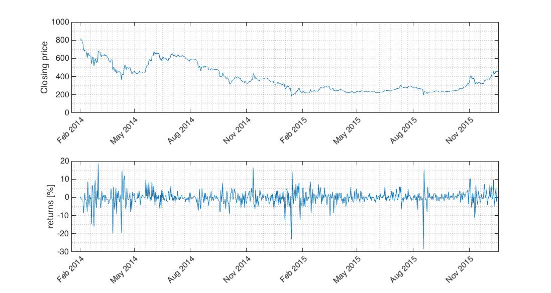
Fig.1 Volatility clusters in returns series are obvious at the first glance.

Let’s examine character of returns mean. Is $\mu_t$ conditioned by its lagged values? ACF, PACF and Ljung-Box test^[5] help us in this decision. Note that $r_t$ series is stationary with mean $\mu_t$ very close to zero. We could use everywhere just $r_t$ instead of innovations $e_t$ but correct is to use innovations/residuals.

%% Autocorrelation of returns innovations - ACF, PACF, Ljung-Box test
% ACF
figure2 = figure;
subplot3 = subplot(2,1,1,'Parent',figure2);
hold(subplot3,'on');
autocorr(e); % input to ACF are innovations after simple linear regression of returns
% PACF
subplot4 = subplot(2,1,2,'Parent',figure2);
hold(subplot4,'on');
parcorr(e); % input to ACF are innovations after simple linear regression of returns
% Ljung-Box test
[hLB,pLB] = lbqtest(e,'Lags',3);

acf_pacf

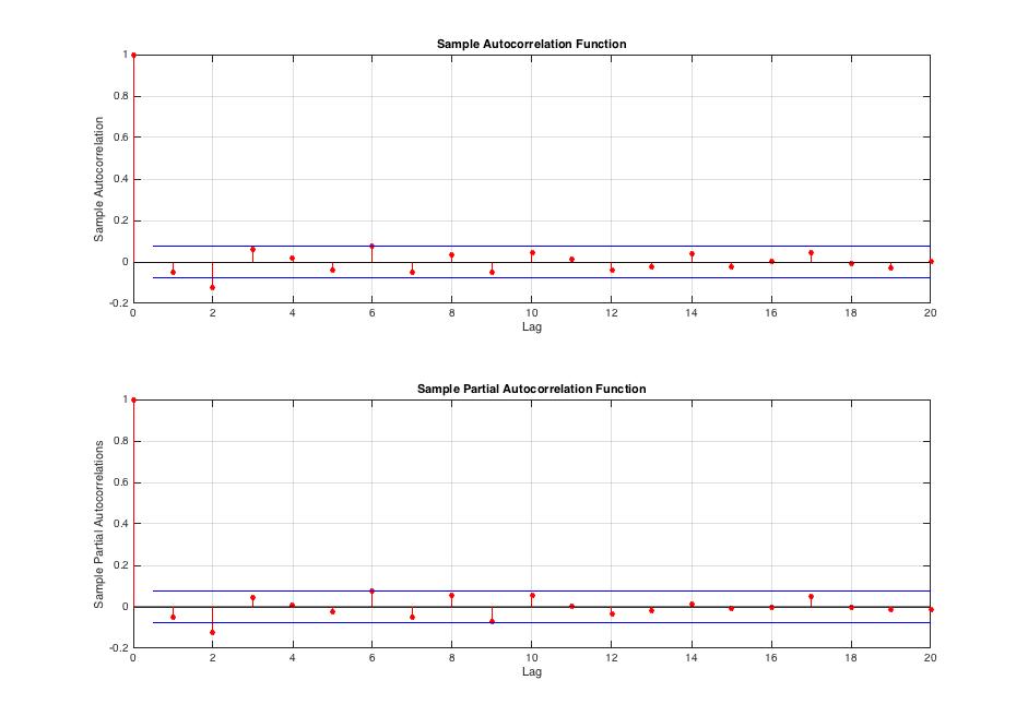
Fig.2 Returns innovation series exhibits autocorrelation at $L=2$

ACF and PACF show us that returns are autocorrelated. We can also reject Ljung-Box test $H_0$ hypothesis with $p \text{-value} = 0.0023$ ^[6] thus there is at least one non-zero correlation coefficient in $\left\{\>\rho(1),\>\rho(2),\>\rho(3)\>\right\}$ .

Next we will check for conditional heteroskedasticity of returns by examining autocorrelation of squared innovations $e_t^2\>$ .

%% Conditional heteroskedasticity of returns - ACF, PACF, Engle's ARCH test
% ACF
figure3 = figure;
subplot5 = subplot(2,1,1,'Parent',figure3);
hold(subplot5,'on');
autocorr(e.^2);
% PACF
subplot6 = subplot(2,1,2,'Parent',figure3);
hold(subplot6,'on');
parcorr(e.^2);

ch_acf_pacf

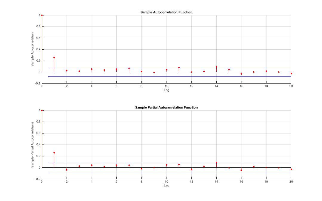
Fig.3 Squared innovation series exhibits autocorrelation at $L=1$ which tells us that variance of returns is significantly autocorrelated thus returns are conditionally heteroskedastic.

Let assure ourselves by conducting Engle’s ARCH test^[7].

% ARCH test
 [hARCH, pARCH] = archtest(e,'lags',2);

ARCH test rejects $H_0$ with ridiculously small $p \text{-value}$ in favor of the $H_1$ hypothesis so returns innovations $e_t$ are autocorrelated – returns are conditionally heteroskedastic. Consider $3,4,5,6,\cdots$ as ‘lags’ input into the ARCH test. What do we expect $p \text{-values}$ to be? Bigger lag we choose, bigger $p \text{-values}$ we can expect. It is naturally caused by that we include more and more values that are not significantly autocorrelated in the ARCH test therefore probability of not-rejecting $H_0$ grows.

Here we go, we made sure that we can apply (1) to given data. After slight modification we have

$r_t = \mu_t + e_t\>,\hspace{5pt} e_t = \sigma_t \>\varepsilon_t \hspace{5pt}.$

where $\mu_t$ is conditional mean and $e_t$ is conditional innovation. We describe our $r_t$ by AR-GARCH models by setting up the ARIMA model objects.

%% AR-GARCH model, ARIMA object
MdlG = arima('ARLags',2,'Variance',garch(1,1)); % normal innovations
MdlT = arima('ARLags',2,'Variance',garch(1,1)); % t-distributed innovations
MdlT.Distribution = 't';

This model corresponds to

(5) $\begin{equation*} r_t = \underbrace{c + \varphi_1 r_{t-1} + \varphi_1 r_{t-2}}_{\mu_t} + \underbrace{\sigma_t\>\varepsilon_t}_{e_t} \end{equation*}$

(6) $\begin{equation*} \sigma_t^2 = \alpha_0 + \alpha_i \> e_{t-1}^2 + \beta_i \> \sigma_{t-1}^2 \hspace{5pt} \end{equation*}$

where we suppose that $\varepsilon_t$ is $\varepsilon_t \sim N(0,1)$ or $\varepsilon_t \sim t(\nu)$ and i.i.d. We will compare quality of both models using information criterions.

Let’s proceed to parameters estimation.

%% Parameters estimation
% normal innovations
EstMdlG = estimate(MdlG,r);
% t-distributed innovations
EstMdlT = estimate(MdlT,r);

gives us following results for normally distributed innovations:

    ARIMA(2,0,0) Model:
    --------------------
    Conditional Probability Distribution: Gaussian

                                  Standard          t     
     Parameter       Value          Error       Statistic 
    -----------   -----------   ------------   -----------
     Constant     -0.0567801      0.172784      -0.328618
        AR{2}     -0.0656668     0.0493691       -1.33012
 
 
    GARCH(1,1) Conditional Variance Model:
    ----------------------------------------
    Conditional Probability Distribution: Gaussian

                                  Standard          t     
     Parameter       Value          Error       Statistic 
    -----------   -----------   ------------   -----------
     Constant        1.30152      0.216776        6.00402
     GARCH{1}       0.831643       0.02415        34.4366
      ARCH{1}      0.0868795     0.0155263        5.59563

Hence we can rewrite (5) and (6) as

$r_t = -0.0568 - 0.0657 r_{t-2} + \underbrace{\sigma_t\>\varepsilon_t}_{e_t}$

$\sigma_t^2 = 1.3015 + 0.0868 \> e_{t-1}^2 + 0.8316 \>\sigma_{t-1}^2$

where we have just one unknown – volatility or conditional variance of returns $\sigma_t^2$ which we can recursively infer. We found out that $\varphi_1=0$ in (5) thus has no explanatory power for returns as dependent variable. Moreover it seems that innovations autocorrelation is not strong enough to give statistical significance to $\varphi_2$ in (5) and to $c$ . T-test^[8] t-statistic for $c$ and $\varphi_2$ don’t fall into the critical region so we can’t reject hypothesis about zero explanatory power of these two coefficients.

For innovations from $t$ -distribution we get:

    ARIMA(2,0,0) Model:
    --------------------
    Conditional Probability Distribution: t

                                  Standard          t     
     Parameter       Value          Error       Statistic 
    -----------   -----------   ------------   -----------
     Constant     -0.0651421     0.0895812      -0.727185
        AR{2}     -0.0728623     0.0350649       -2.07793
          DoF        2.78969      0.325684        8.56564
 
 
    GARCH(1,1) Conditional Variance Model:
    ----------------------------------------
    Conditional Probability Distribution: t

                                  Standard          t     
     Parameter       Value          Error       Statistic 
    -----------   -----------   ------------   -----------
     Constant        1.33968      0.575195        2.32909
     GARCH{1}       0.742378     0.0554331        13.3923
      ARCH{1}       0.257622      0.102234        2.51993
          DoF        2.78969      0.325684        8.56564

Hence we can rewrite (5) and (6) as

$r_t = -0.0651 - 0.0729 r_{t-2} + \underbrace{\sigma_t\>\varepsilon_t}_{e_t}$

$\sigma_t^2 = 1.3397 + 0.2576 \> e_{t-1}^2 + 0.7423 \>\sigma_{t-1}^2$

where $\varepsilon_t \sim t(3)$ . In this case all estimated parameters except of $c$ have statistical significance.

We can also try to model variance using just pure GARCH(1,1) with constant $\mu_t = 0$ in (5) .

%% GARCH without mean offset (\mu_t = 0)
% normally distributed innovations
EstMdlMdloffset0G = estimate(Mdloffset0G,r);
% t-distributed innovations
EstMdlMdloffset0T = estimate(Mdloffset0T,r);

We get similar results as with AR-GARCH approach because AR(2) plays insignificant role in AR-GARCH:

    GARCH(1,1) Conditional Variance Model:
    ----------------------------------------
    Conditional Probability Distribution: Gaussian

                                  Standard          t     
     Parameter       Value          Error       Statistic 
    -----------   -----------   ------------   -----------
     Constant        1.35151      0.219309        6.16257
     GARCH{1}       0.824422      0.024637        33.4627
      ARCH{1}      0.0918974     0.0164784        5.57683

    GARCH(1,1) Conditional Variance Model:
    ----------------------------------------
    Conditional Probability Distribution: t

                                  Standard          t     
     Parameter       Value          Error       Statistic 
    -----------   -----------   ------------   -----------
     Constant        1.30701      0.549996         2.3764
     GARCH{1}       0.740395     0.0547972        13.5115
      ARCH{1}       0.259605      0.100135        2.59256
          DoF        2.82167      0.329997        8.55058

So which model choose now? Model with $t$ -distributed innovations seems to be promising. Let’s examine it quantitatively by AIC^[9], BIC^[10]. Before we can compare our models we need to infer log-likelihood objective functions for each of the model. We can also extract final conditional variances – volatilities.

%% Infering volatility and log-likelihood objective function value from estimated AR-GARCH model
[~,vG,logLG] = infer(EstMdlG,r);
[~,vT,logLT] = infer(EstMdlT,r);

%% Comparing fitted models using AIC, BIC
% AIC,BIC
% inputs: values of loglikelihood objective functions for particular model, number of parameters
% and length of time series
[aic,bic] = aicbic([logLG,logLT],[5,6],length(r))

we get

aic =

3752.3348 3485.1211

bic =

3774.9819 3512.2976

So both AIC and BIC indicate that AR-GARCH with $t$ -distributed innovations should be chosen.

Now we specify and estimate AR-GJR-GARCH adjusting for asymmetric volatility responses and compare it with better performing AR-GARCH with $t$ -distributed innovations using AIC and BIC. We will define just version with $t$ -distributed innovations.

%% AR-GJR-GARCH, ARIMA object
MdlGJR_T = arima('ARLags',2,'Variance',gjr(1,1));
MdlGJR_T.Distribution = 't';

%% Parameters estimation
% t-distributed innovations
EstMdlGJR_T = estimate(MdlGJR_T,r);
    ARIMA(2,0,0) Model:
    --------------------
    Conditional Probability Distribution: t

                                  Standard          t     
     Parameter       Value          Error       Statistic 
    -----------   -----------   ------------   -----------
     Constant     -0.0784738     0.0895587      -0.876227
        AR{2}     -0.0714758     0.0347855       -2.05476
          DoF        2.77131      0.325323        8.51864
 
 
    GJR(1,1) Conditional Variance Model:
    --------------------------------------
    Conditional Probability Distribution: t

                                  Standard          t     
     Parameter       Value          Error       Statistic 
    -----------   -----------   ------------   -----------
     Constant        1.34392      0.580147        2.31653
     GARCH{1}        0.74785     0.0542454        13.7864
      ARCH{1}       0.201164     0.0961537        2.09211
  Leverage{1}       0.101972      0.113445       0.898867
          DoF        2.77131      0.325323        8.51864
%% Infering volatility from estimated AR-GJR-GARCH model
[~,v_GJR_G,logL_GJR_G] = infer(EstMdlGJR_T,r);

%% Comparing fitted models using BIC, AIC
[aic2,bic2] = aicbic([logLT,logL_GJR_G],[6,7],length(r));

we get

aic2 =

          3483.12113743012          3483.95446404909


bic2 =

          3505.76823162144          3511.13097707866

therefore original AR-GARCH slightly outperforms AR-GJR-GARCH. Actually it is obvious from the output of AR-GJR-GARCH estimate because leverage coefficient is statistically insignificant.

Our resulting conditional mean and variance model is AR-GARCH with $t$ -distributed innovations $e_t$ in the following form

$r_t = - 0.0729 r_{t-2} + \underbrace{\sigma_t\>\varepsilon_t}_{e_t}$

$\sigma_t^2 = 1.3397 + 0.2576 \> e_{t-1}^2 + 0.7423 \>\sigma_{t-1}^2$

Let’s plot closing prices along with AR-GARCH with $t$ -distributed innovations and AR-GARCH with normally distributed innovations.

%% plot results
% Closing prices
figure4 = figure;
subplot7 = subplot(2,1,1,'Parent',figure4);
hold(subplot7,'on');
plot(date,C);
ylabel('Closing price');
set(subplot7,'FontSize',16,'XMinorGrid','on','XTickLabelRotation',45,'YMinorGrid','on','ZMinorGrid',...
    'on');
% volatility AR-GARCH, innovations t-distributed
subplot8 = subplot(2,1,2,'Parent',figure4);
hold(subplot8,'on');
plot(date,vT);
% volatility AR-GARCH, innovations normally distributed
plot(date,vG);
ylabel('volatility');
legend({' -distributed',' normally distributed'},'Interpreter','latex');
set(subplot8,'FontSize',16,'XMinorGrid','on','XTickLabelRotation',45,'YMinorGrid','on','ZMinorGrid',...
    'on');

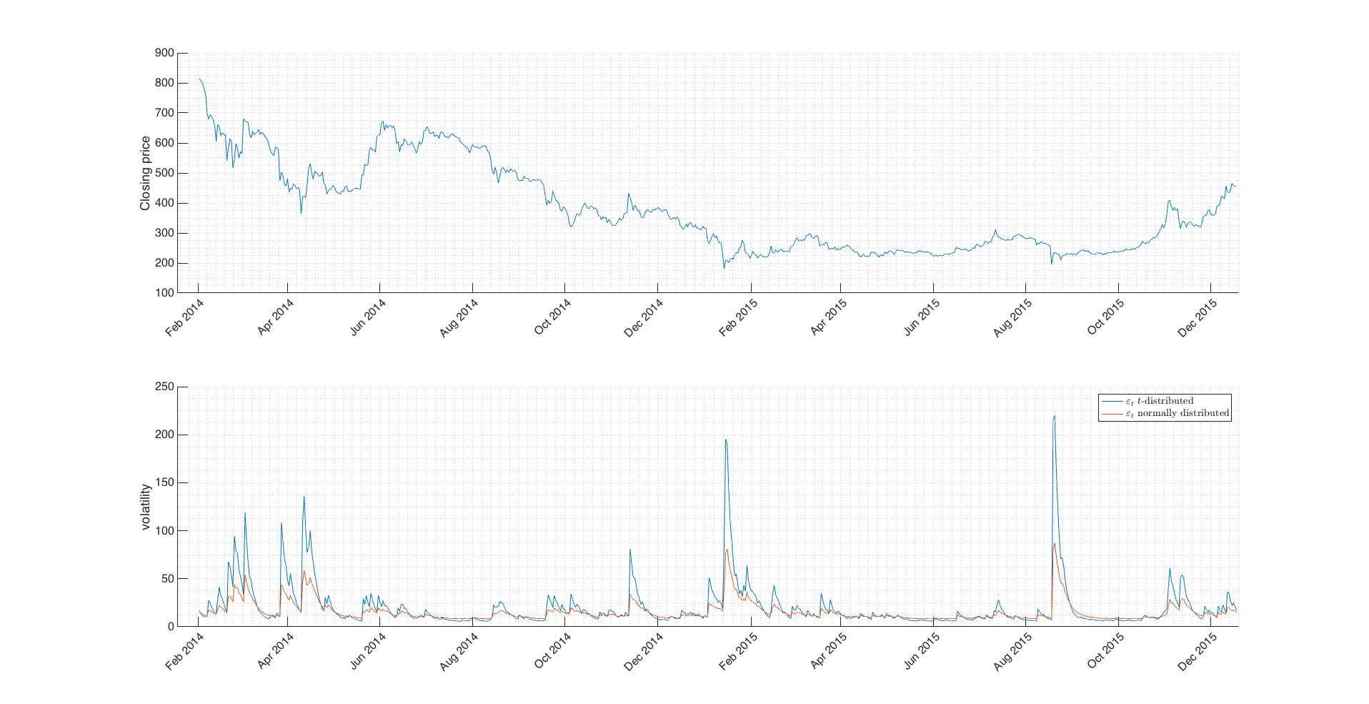
Fig.4 Comparison of generated volatilities. Difference between $\varepsilon_t$ distributions is obvious.

Download all code in one in GARCHestimation.m matlab script.

1. Excess kurtosis

For purpose of this text we consider excess kurtosis as

$\gamma_2 = \frac{E[(X-\mu)^4]}{(E[(X-\mu)^2])^2} - 3 = \frac{\mu_4}{\sigma^4} - 3$

where $\mu_4$ is fourth centered moment about the mean and $\sigma^4$ is clearly squared variance of $X$ . PDF of the random variable $X \sim N(\mu,\sigma^2)$ with $\gamma_2<0,\gamma_2=0,\gamma_2>0$ is respectively said to be platykurtic, mesokurtic or leptokurtic. ARCH models allow for leptokurtic distributions of innovations and returns.

2. $\sigma$ -algebra

Suppose we have a vector of variances $\sigma^2 = (\sigma^2_{t-1}, \sigma^2_{t-2},\cdots)$ and a vector of values of dependent variable $y = (y_{t-1}, y_{t-2},\cdots)$ . Let $t$ denote time. We can state that these two vectors contain information. Now consider arbitrary functions $f(\sigma^2,y)$ , then information generated by $f$ is considered to be $\sigma$ -algebra generated by given set of vectors. So if we have whatever conditional variable it just means that we suppose its value is dependent on some other values through a function.

3. AR process

Auto-regressive process AR(p) is defined as

$y_t = \varphi_1 y_{t-1} + \cdots + \varphi_p y_{t-p} + \varepsilon_t\hspace{5pt}.$

After slight modification we can us AR(p) as

$r_t = \varphi_1 y_{t-1} + \cdots + \varphi_p y_{t-p} + e_t\hspace{5pt}.$

4. Just common denotations for one value, take a think just about last equality.

5. Ljung-Box test

Test whether any of a given group of autocorrelations of a time series are different from zero.
$H_0$ : The data are independently distributed (up to specified lag $L$ ).
$H_1$ : The data are not independently distributed. Some autocorrelation coefficient $\rho(k)=1,\cdots,L$ is non-zero.

6. $\text{p-value}$

Familiar $\text{p-value}$ discussed by many students and practitioners forevermore. There are many intuitive interpretations of this value, some of them correct some of them not. I recommend you find your one which fits your mind best. For me personally it’s “the greatest significance level up to which we would not reject the null hypothesis”. Sometimes it’s being said to be plausibility because less $\text{p-value}$ is, less acceptable null hypothesis is.

7. Engle’s ARCH test

Engle’s ARCH test assess the significance of ARCH effects in given time-series. Time-series of residuals doesn’t need to be autocorrelated but can be autocorrelated in squared residuals, if so, we get familiar ARCH effect. Note that innovations figure as residuals.
$H_0$ : The squared residuals are not autocorrelated – no ARCH effect.
$H_1$ : The squared residuals are autocorrelated – given time-series exhibits ARCH effect.

8. T-test

We use one-sample T-test with hypotheses defined as
$H_0: \beta = 0$ .
$H_1: \beta \ne 0$ .
where $\beta$ is parameter in question.

9. AIC

Akaike’s Information Criterion (AIC) provides a measure of model quality. The most accurate model has the smallest AIC.

10. BIC

The Bayesian information criterion (BIC) or Schwarz criterion is a criterion for model selection among a finite set of models, the model with the lowest BIC is preferred.

MMquant