Introduction to volatility models with Matlab (SMA, EWMA, C-C, Range estimators)

In this article I will introduce some of the tools used to model volatility with examples in Matlab. Let’s start with a definition of volatility –

Volatility is the degree of variation of a price series over time as measured by the standard deviation of returns.

Why is volatility of vast importance in financial world? One of the main reason is because it’s used as a measure of risk. Greater volatility of an asset means riskier opportunity for potential investor and vice versa. In practice traders can use output from volatility models to set up leverage(or any other parameter) of their positions thus volatility can help optimize a trading strategy. Usually PnL of a trading strategy is a function of volatility or at least variance of PnL is. We can explore such a volatility-PnL relation via regression analysis but it’s not aim of this article.

Historical volatility

Sometimes called realized volatility or simple moving average(SMA). The historically oldest approach to volatility comes directly from the definition. We just select rolling window of length $k$ over time serie and calculate volatility as sample variance of returns over given period $k$ from time $t-k$ to $t-1$ . That is

(1) $\begin{equation*} \hat{\sigma}_t^2 = \frac{1}{k-1}\sum \limit _{\tiny \tau=t-k}^{\tiny t-1}(r_\tau - \hat{\mu}_t)^2 \end{equation*}$

where $\hat{\mu}_t$ is simply sample mean of returns over given period $k$ calculated over same window from $t-k$ to $t-1$

$\hat{\mu}_t = \frac{1}{k}\sum \limit _{\tiny \tau=t-k}^{\tiny t-1}r_\tau$

and $r_\tau$ is particular asset return over one time unit

$r_\tau = ln \bigg(\frac{p_{\tau}}{p_{\tau-1}}\bigg)\hspace{5pt}.$

Observe that this model has one big disadvantage of assigning equal weights to terms in sum in (1). Suppose there was some short-term significant swing in volatility at time $t_0$ . Then every calculation of $\hat{\sigma}_t^2$ from time $t_0$ to time $t_0+k$ will contain this outlier with same weight. This will cause plateauing of such an estimate. Download function for $\hat{\sigma}_t^2$ calculation here. I will demonstrate the plateauing effect on bitcoin daily price time serie.

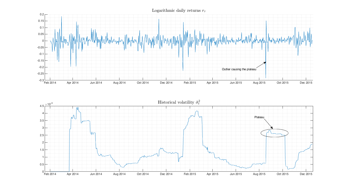Plateau Fig.1 On these two plots we can see that sudden fluctuation of returns causes the plateauing effect and the model gives strongly biased volatility estimate.

The market convention is to quote in terms of annualized volatility. For daily historical volatility we have $\hat{\sigma}_{t,1d} = \sqrt{\hat{\sigma}_t^2}$ and we can annualize it as $\hat{\sigma}_{t,1y} = \sqrt{252}\hspace{2pt}\hat{\sigma}_{t,1d}$ .

If we slightly modify the (1) considering $\hat{\mu}_t = 0$ we get rid of one estimation. This can be clearly done just for series of logarithmic returns, not for price series. Thus we get simple close-close volatility estimator

$\hat{\sigma}_t^2 = \frac{1}{k-1}\sum \limit _{\tiny \tau=t-k}^{\tiny t-1}r_\tau^2 \hspace{5pt}.$

cc_vs_nocc

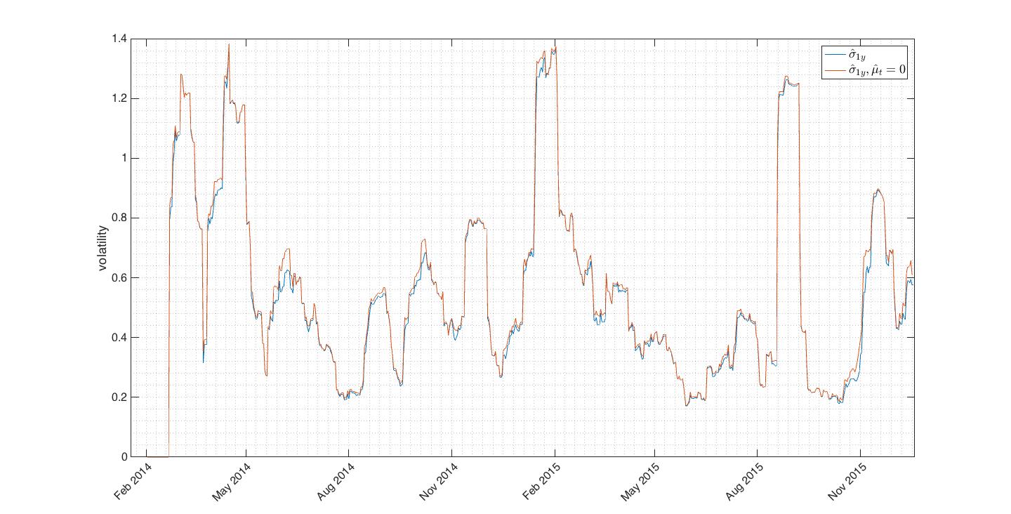
Fig.2 Comparison of SMA and SMA with close-close approach. Both estimates follows tightly each other.

EWMA model

EWMA model is extented version of forementioned simple historical volatility and partial solution to the plateauing issue. EWMA approach was developed by J.P.Morgan within the RiskMetrics methodology framework and is defined as follows

(2) $\begin{equation*} \hat{\sigma}_t^2 = (1-\lambda )\sum \limit _{\tiny j=0}^{\tiny \infty}\lambda^j (y_{t-1-j}-\overline{y})^2 \end{equation*}$

or after rearranging

(3) $\begin{equation*} \hat{\sigma}_t^2 = (1-\lambda )(y_{t-1}-\overline y)^2 + \lambda \hat{\sigma}_{t-1}^2 \end{equation*}$

where $y$ is an asset price, $\overline{y}$ is mean of an asset price and $\lambda$ is decay factor such that $0<\lambda<1$ . In (2) note that as $j \rightarrow \infty$ we have $\lambda^0 > \lambda^1 > \lambda^2 > \cdots$ or $\lambda \rightarrow 0$ so deeper observations get smaller and smaller weights.

If we want EWMA model for logarithmic returns we just swap $y$ in (2) and (3) for $r$ and in practice we can drop the $\overline r$ term after we checked that $\overline r = 0$ holds. Hence we get

$\hat{\sigma}_t^2 = (1-\lambda )r_{t-1}^2 + \lambda \hat{\sigma}_{t-1}^2 \hspace{5pt}.$

Observe how $1-\lambda$ and $\lambda$ weight terms in the model. Greater $\lambda$ makes model more affected by last variance, in other words model tends to revert to its previous volatility level(variance). Conversely small $\lambda$ gives more weight to last return. $\lambda$ is sometimes called memory because it directly affects how much is variance dependent on its previous value. RiskMetrics methodology suggest use $\lambda = 0.94$ which is widely used by practitioners.

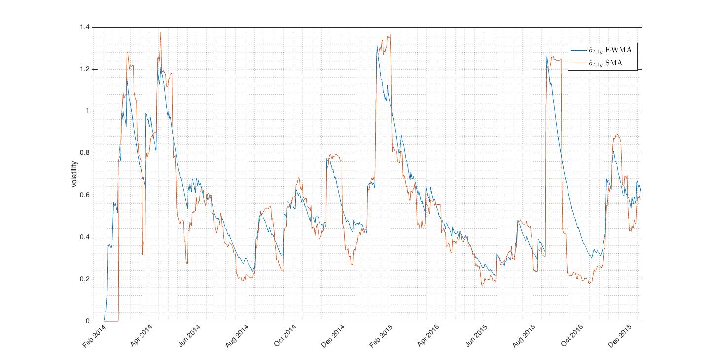Fig.3 Exponentially decaying EWMA is still biased by outliers but gives much better volatility estimate than SMA.

You can download Matlab function for EWMA volatility estimate here.

Parkinson estimator

In 1980, a physicist Michael Parkinson showed in his paper that we can project additional information to volatility estimate by using not just close prices but rather price extremes. He proposes use of log differences between highs and lows over specified time window. Such an estimator is five times more efficient than historical SMA approach (for same amount of input data PE variance is 1/5th of SMA variance). Rolling PE is given by

$\hat\sigma_t^2 = \frac{1}{4\>k\>ln(2)} \sum \limit _{\tiny \tau=t-k}^{\tiny t-1} ln^2 \left( \frac{H_\tau}{L_\tau}\right)$

where $\hat\sigma_t$ is PE volatility computed over given time window $t-k$ to $t-1$ and $H_\tau,L_\tau$ are corresponding high and low.

PE_vs_SMA

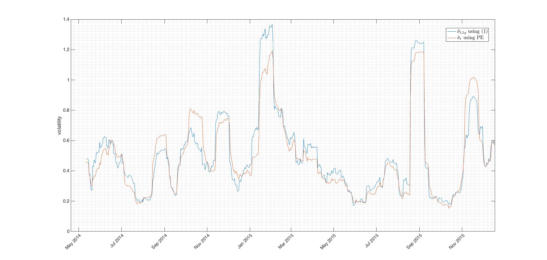
Fig.4 Even that Parkinson estimator is significantly more precise in the term of variance it tends to underestimate volatility as seen on picture above. It should be used in combination with other estimators which don’t underestimate. We can include PE in a volatility composite.

Plots above were made using my PEvol() function.

Garman-Klass estimator

In 1980, Garman-Klass realized that utilizing all of the OHLC information must give even more precise volatility estimation than PE. It can be explained as an optimal (smallest variance) combination of SMA and PE. G-K estimator is 7.4x more efficient than SMA. Considering our rolling window of size $k$ , G-K estimator is written as

(4) $\begin{equation*} \hat\sigma_t^2 = \frac{1}{k} \sum \limit _{\tiny \tau=t-k}^{\tiny t-1}\Big[0.511\hspace{2pt} ln^2\Big(\frac{H_{\tau}}{L_\tau}\Big) - 0.019\hspace{2pt} ln\Big(\frac{C_\tau}{O_\tau}\Big)\>ln\Big(\frac{H_\tau L_\tau}{O^2_\tau}\Big) - 2\hspace{2pt}ln\Big(\frac{H_\tau}{O_\tau}\Big)\>ln\Big(\frac{L_\tau}{O_\tau}\Big)\Big] \end{equation*}$

where $O_\tau,H_\tau,L_\tau,C_\tau$ are respectively open,high,low,close at time $\tau$ in the particular rolling window. Second term in (4) in the brackets can be neglected since it’s very small.

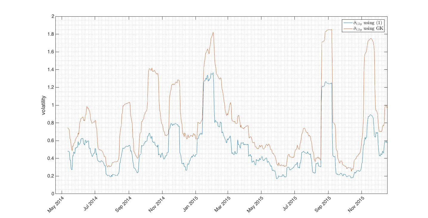
Fig.5 Disadvantage of G-K estimator is that it’s trend dependent. As we used bitcoin price data with strong drift the G-K estimation gives overestimated volatility values.

Download Matlab function for Garman-Klass estimation.

Rogers – Satchell

R-S volatility estimator was published in 1991. This estimator is independent of the drift and computed as

(5) $\begin{equation*} \hat\sigma_t^2 = \frac{1}{k} \sum \limit _{\tiny \tau=t-k}^{\tiny t-1}\Big[ln\Big(\frac{H_{\tau}}{C_\tau}\Big)\>ln\Big(\frac{H_{\tau}}{O_\tau}\Big) + ln\Big(\frac{L_{\tau}}{C_\tau}\Big)\>ln\Big(\frac{L_{\tau}}{O_\tau}\Big)\Big] \hspace{5pt}. \end{equation*}$

sma_rs

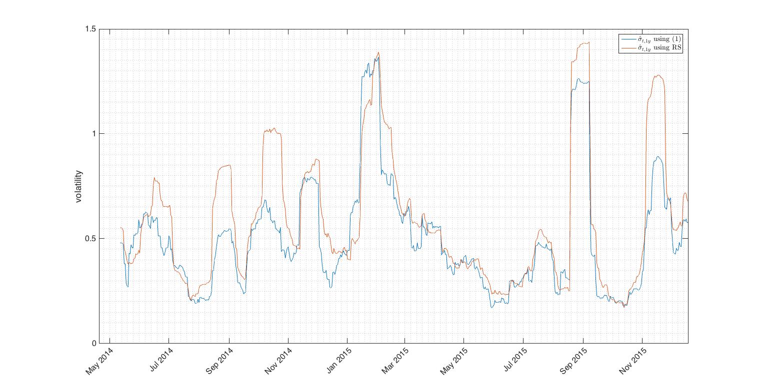
Fig.6 R-S estimator closely follows SMA estimate during low volatility periods. Difference of estimators during volatility peaks is due to the wide trading ranges in these periods and lack of SMA estimator incorporate this fact.

Matlab function for R-S estimate can be downloaded here.

Discussion above shows that historical volatility estimators can be sorted into

mean-deviation estimators (SMA, EWMA)
close-close estimators (SMA( $\hat{\mu}_t = 0$ ), EWMA( $\hat{\mu}_t = 0$ ))
range estimators (P-E, G-K, R-S).

Great paper on properties of range-based estimators with further details can be downloaded here.

MMquant